# Function to calculate PR curve data using PRROC
calculate_pr <- function(model, test_data, true_labels, positive_class) {
pred_probs <- predict(model, newdata = test_data, type = "prob")[, positive_class]
true_binary <- ifelse(true_labels == positive_class, 1, 0)
pr <- pr.curve(scores.class0 = pred_probs, weights.class0 = true_binary, curve = TRUE)
return(pr)
}
# Calculate PR curves
pr_glm <- calculate_pr(glm.fit, data.tst, data.tst$Class, "malignant")
pr_knn <- calculate_pr(knn.fit, data.tst, data.tst$Class, "malignant")
pr_lda <- calculate_pr(lda.fit, data.tst, data.tst$Class, "malignant")
pr_qda <- calculate_pr(qda.fit, data.tst, data.tst$Class, "malignant")
pr_nb <- calculate_pr(nb.fit, data.tst, data.tst$Class, "malignant")
# Extract AUC-PR values
auc_pr_values <- c(
Logistic = pr_glm$auc.integral,
KNN = pr_knn$auc.integral,
LDA = pr_lda$auc.integral,
QDA = pr_qda$auc.integral,
`Naive Bayes` = pr_nb$auc.integral
)
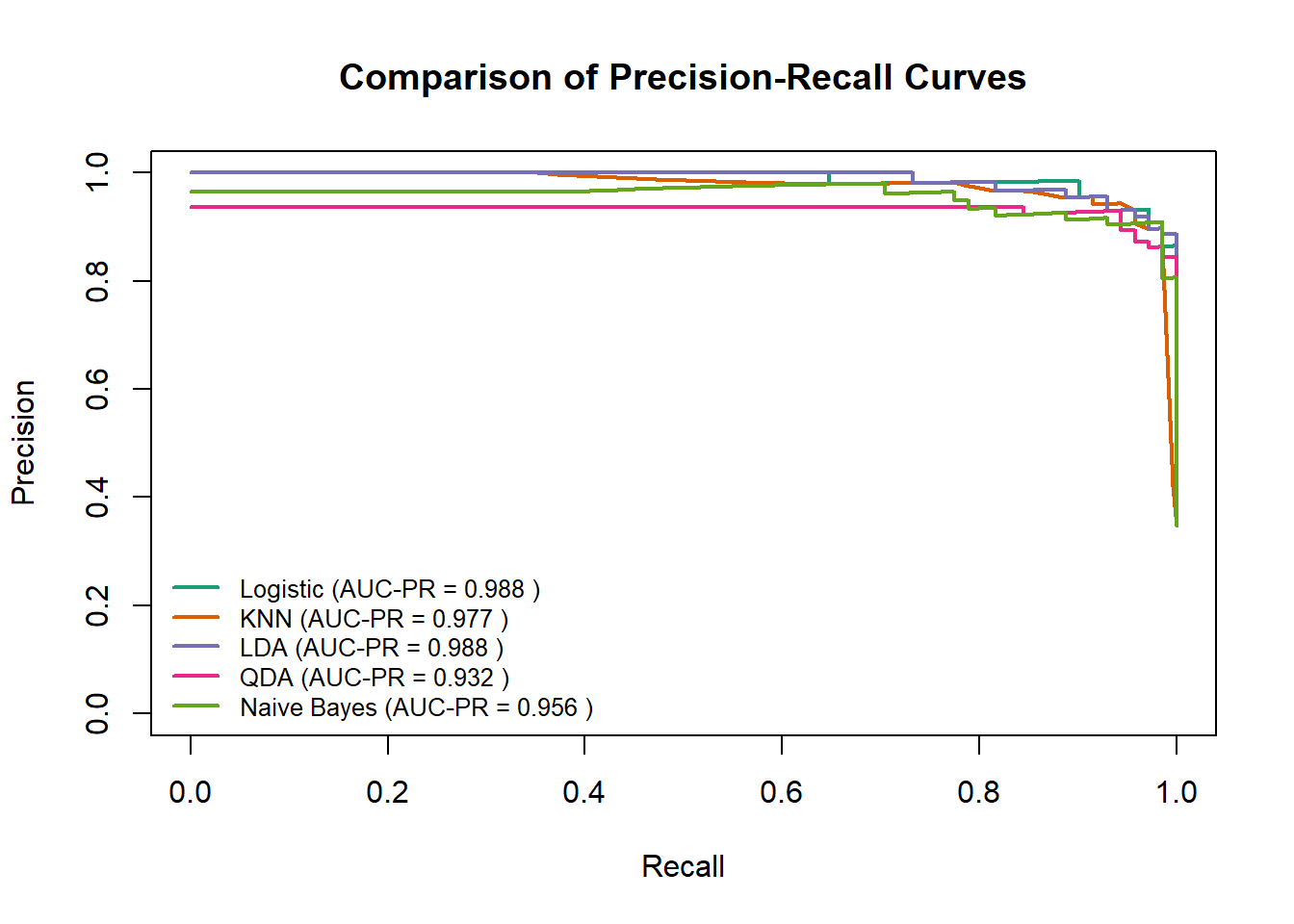
# Plot PR curves using PRROC's plot function
plot(pr_glm, main = "Comparison of Precision-Recall Curves", col = "#1B9E77", lwd = 2, auc.main = FALSE, legend = FALSE)
plot(pr_knn, add = TRUE, col = "#D95F02", lwd = 2, auc.main = FALSE, legend = FALSE)
plot(pr_lda, add = TRUE, col = "#7570B3", lwd = 2, auc.main = FALSE, legend = FALSE)
plot(pr_qda, add = TRUE, col = "#E7298A", lwd = 2, auc.main = FALSE, legend = FALSE)
plot(pr_nb, add = TRUE, col = "#66A61E", lwd = 2, auc.main = FALSE, legend = FALSE)
# Add Legend
legend("bottomleft",
legend = paste(names(auc_pr_values), "(AUC-PR =", round(auc_pr_values, 3), ")"),
col = c("#1B9E77", "#D95F02", "#7570B3", "#E7298A", "#66A61E"),
lwd = 2, cex = 0.8, bty = "n") # bty="n" removes legend box